Chapter 1
A First Model
In this chapter we develop a program that can tell two kinds of points apart. We begin with a single neuron and then build, from layers of neurons, a small network that finds its own weights.
Two Kinds of Points
Let there be a plane with the coordinates
and , each from -6 to +6. Into this plane we put
points of two kinds: orange and blue. In the programs the kind of a
point is represented by a number: 1 for orange and
-1 for blue.
A model is a function that computes, from the coordinates and of a place in this plane, a guess of the kind of a point at that place: a value between -1 and +1. At -1 the model is sure that a blue point lies there; at +1 it predicts an orange one with certainty. Values in between express uncertainty: the sign says which kind the model leans to, and the nearer the value is to 0, the less sure it is; at 0 it cannot decide.
We could write such a function any way we like, for example
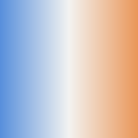
It is +1 at the right edge, -1 at the left and 0 on the upright axis: on the right it guesses orange, on the left blue, and the nearer the middle, the less sure it is. Or
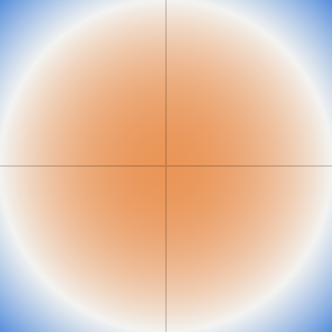
It is +1 at the centre, −1 in the four corners, because there , and 0 on the circle of radius 6 around the centre, where . Whether such a function can predict the points' kinds well depends on where they lie: the first suits points that are orange on the right and blue on the left, the second an orange disc in a blue ring.
Machine learning, on the other hand, does not make the formula up. It fixes only its general form, a formula with numbers left open, the parameters. In the second example the 36 could be such an open number, , and would decide how large the orange disc is; where the formula falls below −1, it counts as −1. Which values the parameters get, a program finds out from examples, points whose kind is known. Finding them is what this book calls learning, and a function with its parameters found a trained model.
One Neuron
The simplest form of such a function is a neuron. It multiplies each of its inputs by a number of its own, its weight, adds them up and adds one more number, its bias:
The result is called the neuron's weighted sum. Where it is positive the neuron guesses orange, where it is negative, blue. The points where is exactly 0 form a straight line, so a neuron parts the plane by a line: the weights turn it, the bias moves it.
Now let us try to adjust the neuron so that it can tell, as well as possible, the colour of six points we scatter over the plane at will: three orange and three blue. We begin with the weights 1 and 1 and the bias 0:
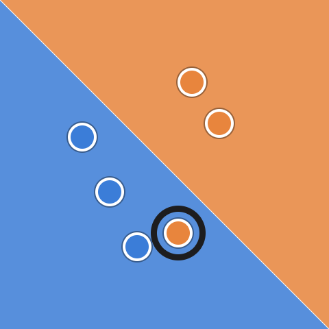
Five of the six lie on the right side; the one in the ring is orange but lies below the line. With the line turns to the upright axis, and all six are right:
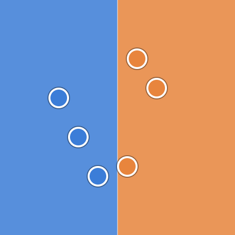
Changing the weights and the bias step by step until the guesses are right is the essence of what we shall call learning.
How Wrong
To change the weights by itself a program needs a measure of how wrong the neuron is. This measure is a number that gets smaller as the neuron gets better. Counting the wrong guesses does not serve: a small change of a weight usually changes no guess at all, so the count does not say which way to turn.
So we first map the weighted sum to a number between −1 and 1 by a smooth function, here the hyperbolic tangent:
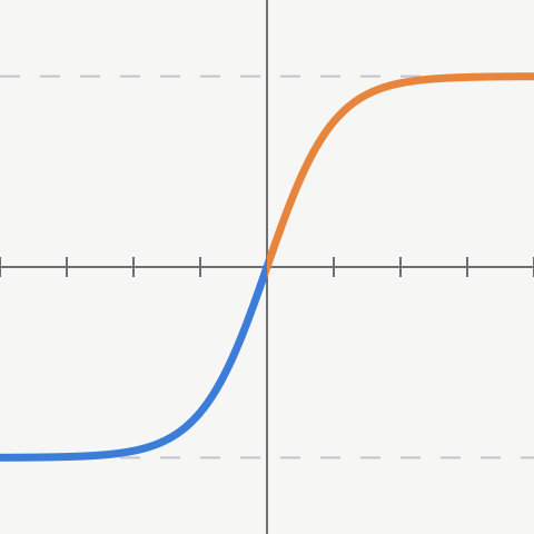
With this function the model can answer as the beginning of the chapter asked: near +1 or -1 where it is sure, near 0 where it is not. Such a function we shall call the neuron's activation function, and its answer for a particular point of the plane. Now the answer can be compared with the kind the point really has:
is the loss of one point: 0 where the answer is exactly the kind, larger the further it is from it, and every small change of a weight changes it a little. The mean of the losses of all points is the neuron's loss, and that is the measure we were looking for.
The hyperbolic tangent is not the only possible activation function. In large networks one mostly takes an even simpler function today, ReLU: , that is itself where is positive and 0 elsewhere. Its slope is always 1 for positive , while that of tanh becomes nearly 0 far out. What that means for learning shows in the next section.
Downhill
So the loss of our neuron is a function of the three values , and . Now we want to find the values for which it becomes as small as possible. Trying every combination is out of the question: each of the three values can be any number, so there are infinitely many. Even if we tried only 100 numbers for each value, that would be , a million combinations, and for each we would have to compute the loss over all points. For three values a computer still manages that, but the network for XOR that we build later already has 13 numbers and so combinations, and large networks have millions of weights. So we begin with some values and move from there step by step in the direction in which the loss falls fastest, with all three values at once. Which direction that is can be read off each value separately: how much does the loss change when the value changes a little? That is the partial derivative of the loss with respect to that value, for written . It is partial because only this one value changes while the others are held fixed; the round instead of a marks that.
The loss does not depend on directly. It depends on the answer , the answer on the sum , and the sum on . Each link of that chain has a derivative that is easy to work out:
How much does the loss change when the answer changes? , the derivative of .
How much does the answer change when the sum changes? , the derivative of tanh.
How much does the sum change when changes? , because is multiplied by .
The chain rule says that the derivative of the whole chain is the product of the derivatives of its links:
For the last factor is , for the bias it is 1. Added up over all points and divided by their number, these partial derivatives are the gradient: the direction in which the loss rises fastest. One step of gradient descent moves each of the three values a little the other way,
where the small number is the learning rate.
And when does one stop? When the loss is small enough, or when it hardly falls any more. The pages of this chapter stop as soon as the loss is below 0.02 or has fallen by less than 0.0001 over a hundred steps. Such a rule is called a stopping criterion.
Try the start values as well (the page with these values): then the neuron hardly moves, and after a hundred steps the page stops, since the loss no longer falls. Nearly all points lie on the wrong side, and far from the line, where tanh is nearly ±1 and hardly rises any more. Since the factor is nearly 0 there, so is the gradient: a neuron that is sure and wrong hardly learns. This is called saturation, and it is why one begins with small weights.
Better Inputs
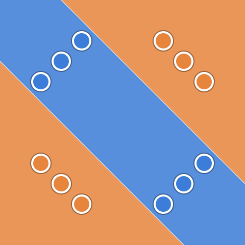
Our neuron parts the plane by a line. But some arrangements of points cannot be parted by a line, for example a disc of orange points inside a ring of blue ones: every line then has orange and blue on both sides.
What the neuron lacks is not skill at sums but the right view of the points. Let us give it the squares of and as its inputs instead:
With and , say, is 0 exactly where , on the circle of radius 3 around the centre. Inside, is positive, outside negative:

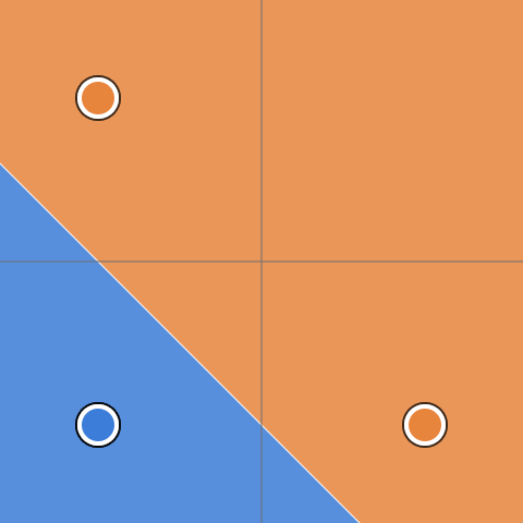
Why can the neuron do this all of a sudden? Let us call its new inputs and . Then is a straight line again, only not in the plane of and but in that of and . Drawn there, the disc lies near the origin and the ring further out, and a line parts them:
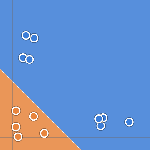
So the neuron still draws a line, but a line in the inputs it is given; on the plane of the points it becomes a circle. Choosing what a model sees is called feature engineering, and good inputs can make a hard problem easy.
Backpropagation
How does a hidden neuron learn? Its weights are as far from the loss as can be, behind the output neuron. The chain rule still works, with a chain one link longer. The clever part is the order in which it is computed.
First everything is computed forward, as before: each hidden neuron's answer , then the output's sum and its answer . Then backward. The output neuron's share of the error, the loss by its sum, is the familiar
and its weights' derivatives follow from it as for a single neuron: for the weight that reads hidden neuron . Hidden neuron reaches the loss through that weight, so its answer's slope is , and through its own tanh its share of the error becomes
From there its weights are once more a single neuron's: , and for its bias. The error is handed back through the network layer by layer, each layer's share computed from the share of the layer after it. That is backpropagation, and it is the whole secret of how networks of any depth learn.
The hidden neurons on the page start from different weights on purpose. Had they all started alike, they would answer alike, get the same gradient in every step and stay alike forever, three copies of one line. That is why a network usually starts from random weights.
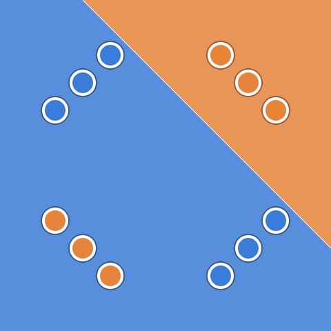
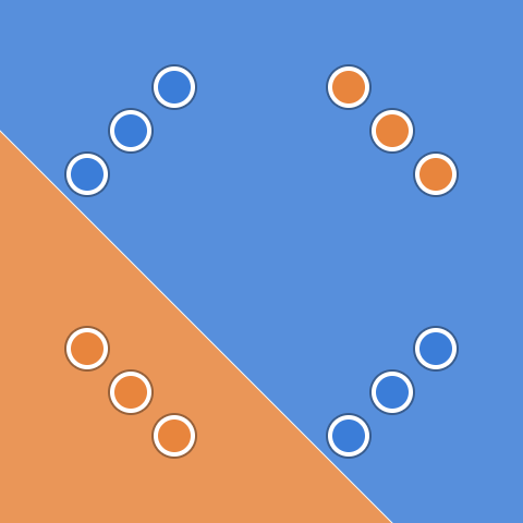
A network needs nothing more to learn, however many layers it has: compute forward, hand the error back, move each weight a little against its gradient. How far that carries shows on the field, a page with a larger network than in our boxes: up to six hidden layers of up to eight neurons, seven inputs to choose from, the squares among them, and four arrangements of points, a spiral among them. For each neuron a small square shows what it answers over the whole plane, like our pictures for XOR.
What It Has Not Seen
A model that knows its training points is not yet useful. The question is how well it guesses points it has never seen. That is why the field holds back half of its points as test points, drawn with a ring: the network never learns from them, and the loss over them, the test loss, says how well it generalizes.
When the data is noisy and the network large, the two losses part ways. The network learns the training points ever better, noise included, and draws borders around single stray points; the test loss stops falling and rises. That is overfitting. One cure is regularization: an extra loss for large weights, for each weight. Its derivative shrinks every weight a little in every step, and a network with smaller weights draws smoother borders.
The Field's Program
The page runs one Scaly program, field.scaly,
built for WebAssembly. It is this chapter's programs grown up: up to
six hidden layers of up to eight neurons, seven inputs to choose
from, four activation functions, regularization, and backpropagation as in
the last section, only in loops over layers instead of written out.
It keeps everything the page shows in one vector of numbers in its
memory, which the page reads directly, without a copy; the picture
of the network's answer over the plane is a for
over its 6400 points, which Scaly spreads over the cores of the
machine by itself. Its source is
on GitHub.
Everything this chapter derived by hand, the chain rule through every link and the gradient of every weight, a program can derive too. That is the subject of the chapters ahead: first how Scaly holds many numbers at once, in tensors, then a tape that records the forward computation and plays it back to get every derivative.